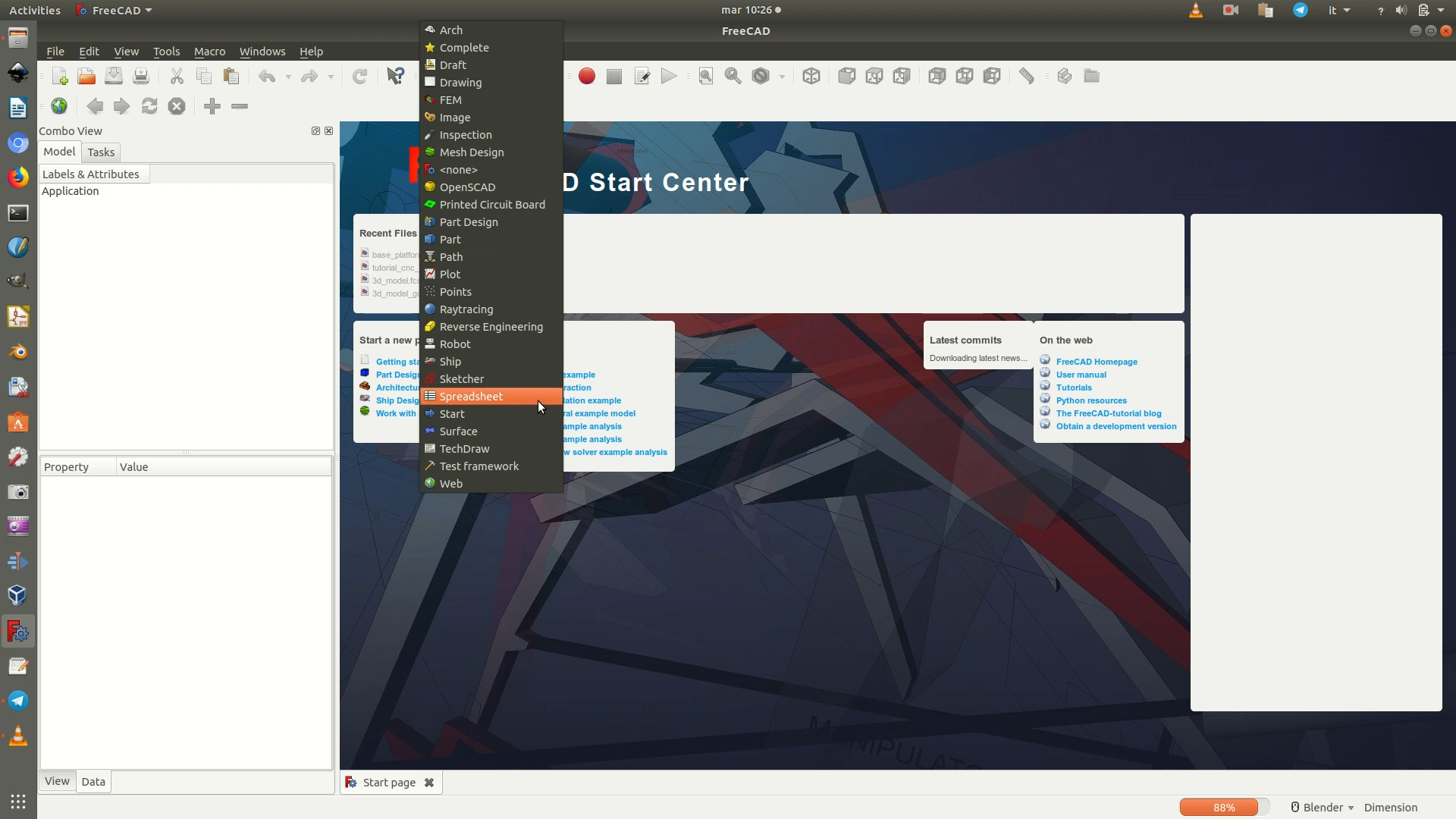
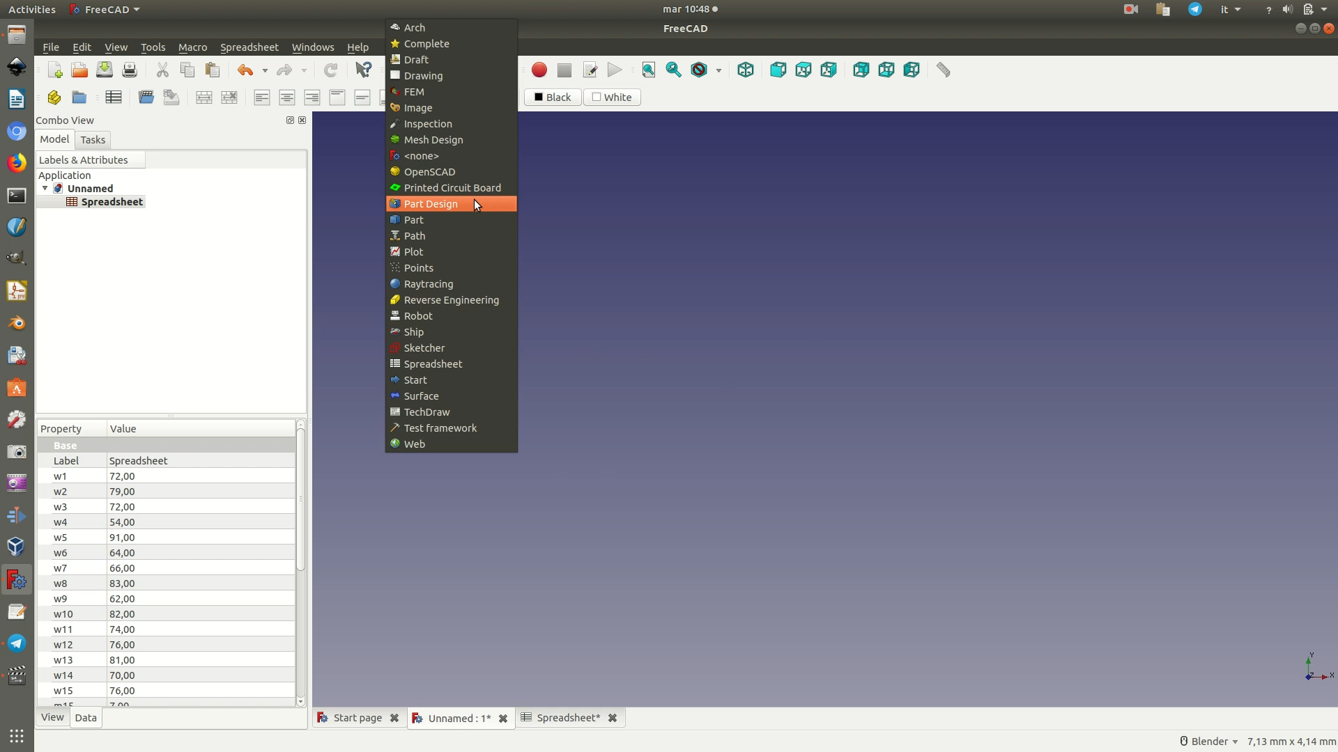
1. After opening FreeCAD and creating a new project by clicking on File > New, open the Spreadsheet Workbench, as shown in the image, by clicking on the dropdown menu where you now see Start. This workbench contains all the commands related to working with data.

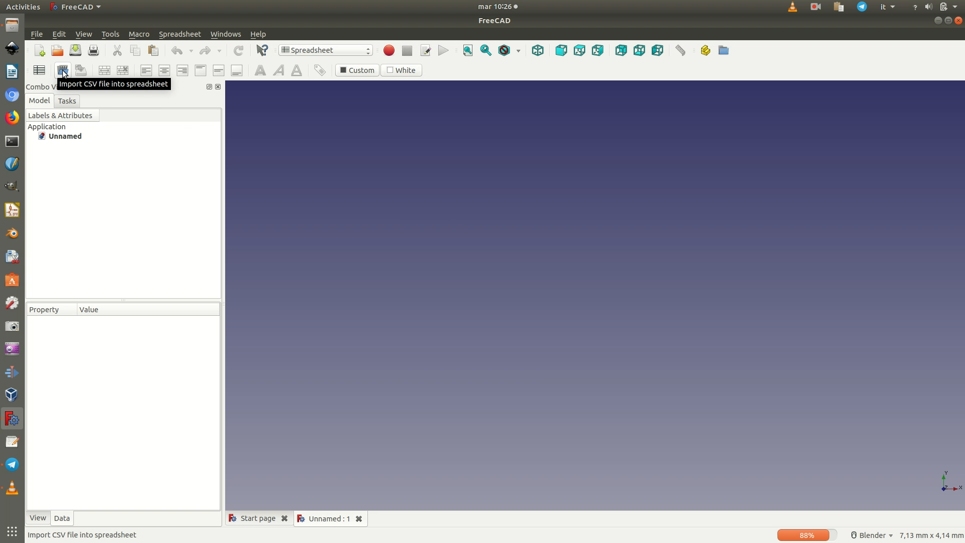
2. Import the data into the project by clicking through File > Open. Data can be in .CSV or .XLSX format. Note on .CSV files: while the file extension has to be .CSV in order for the file to be imported, the data actually has to be in.TSV format (tab-separated, not commas). Otherwise, the columns won't be separated correctly."

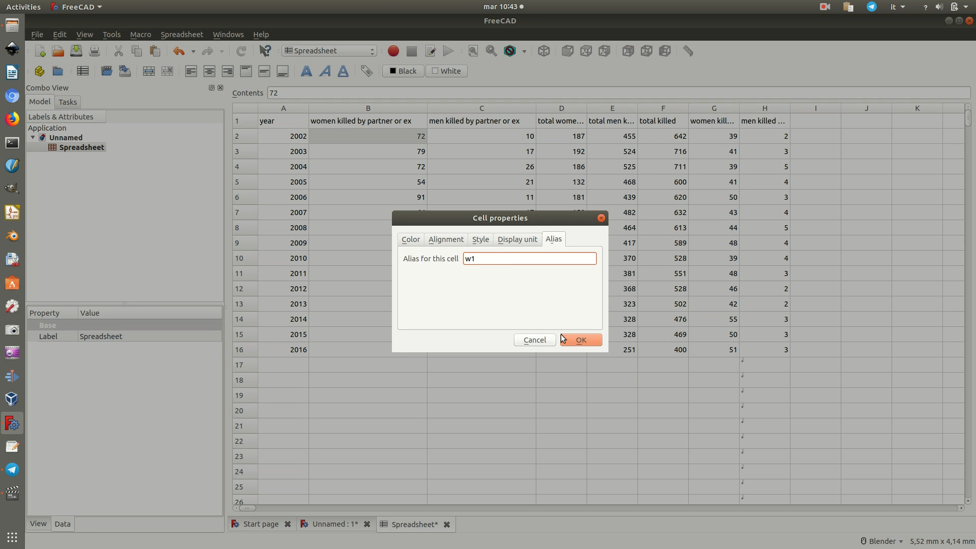
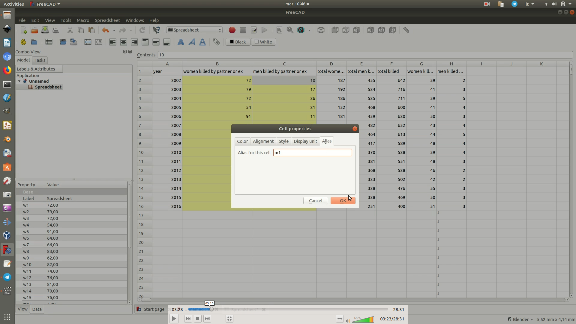
3. Create an alias for each cell. This will allow you to bind each value of the data to a physical characteristic of the object (length, width, etc.). Assigning aliases implies manually clicking on each cell containing the data you want to plot (excluding the header row and the first column with the row names) and typing a label name to reference it by. 
Despite being a manual task, the operation is quite quick. Yet, it will become quite burdensome if your spreadsheet has hundreds of cells or more. In this case you will need to resort to other techniques, like using FreeCAD MACROS and plugins, or going for another software like Blender¹. 
To make things easier on yourself, when choosing the aliases, give meaningful names that follow a logic order (a1, a2, a3; b1, b2, b3; etc.): you will need to reference them again further on. To assign an alias, right-click on a cell and select Properties Then, click on the Alias tab and type in the name. The cell will now be highlighted in yellow.
¹ The easiest way is actually to directly import a 2D .SVG line chart. The technique is not proposed for this tutorial because it is useful to learn how to bind data to object's geometries from scratch, regardless of the shape of the object/chart, so that the same process can be used to produce any data-driven shape. If you wish however to go for the quickest route, in this case you can read and adapt our other tutorial to learn how to import and extrude a .SVG file in FreeCAD (read on from step 7 of the linked tutorial).

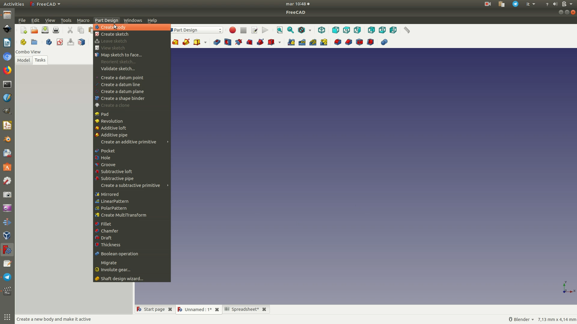
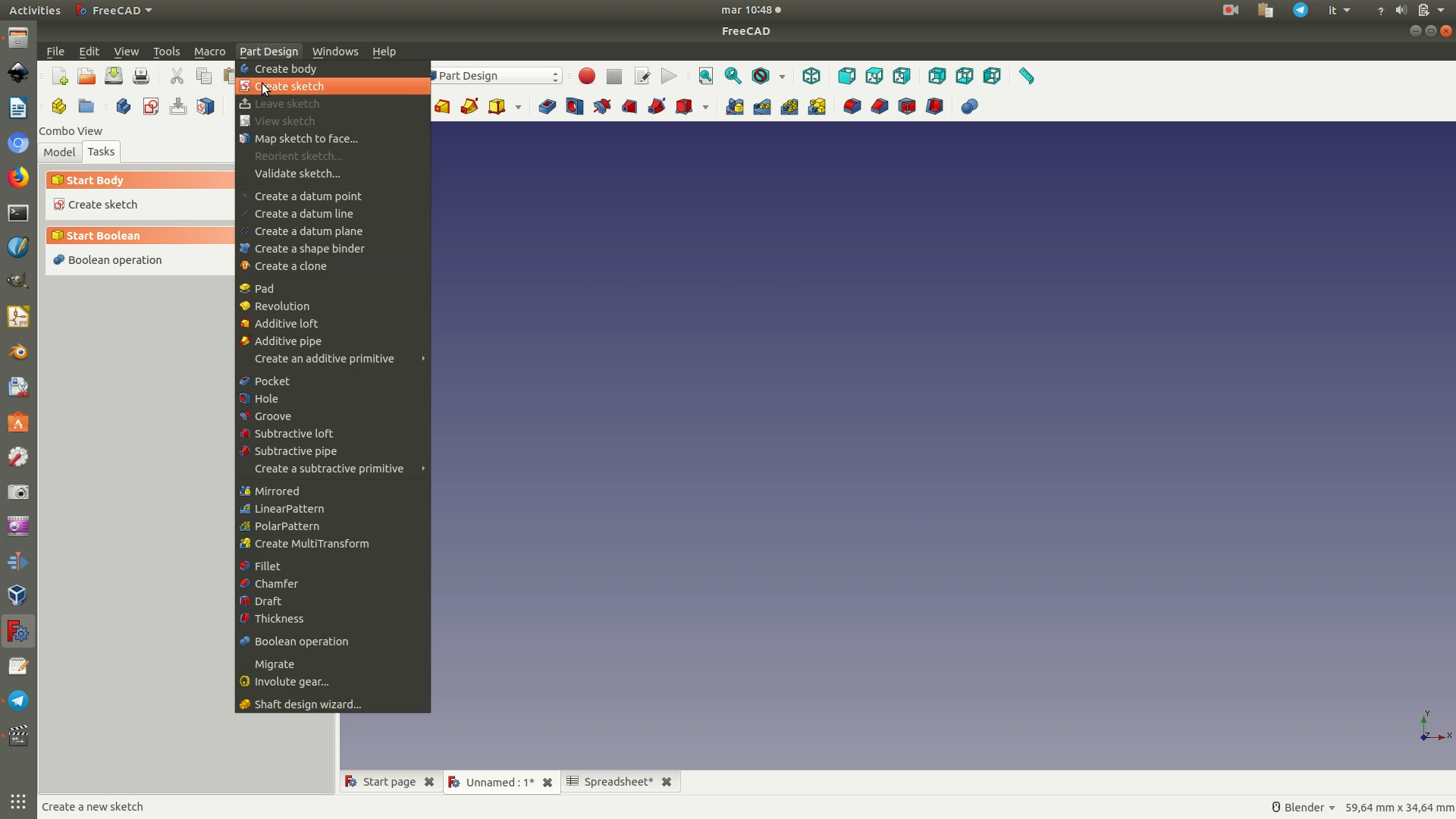
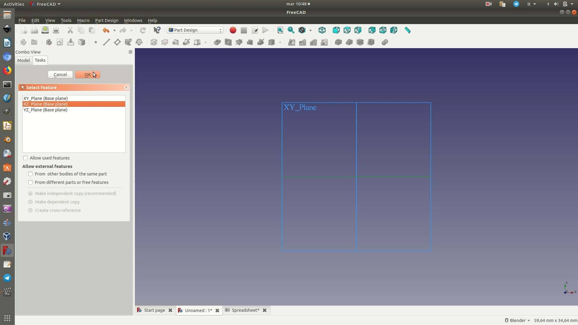
4. Move to the Part Design Workbench by clicking through the dropdown menu where you now see Spreadsheet. This workbench groups all commands used to model the single parts of the object. Once you have opened this workbench, you need to create a new body (the container for your design) and a new sketch (the 2D drawing of your object). To do this, first click through the menu Part Design > Create Body, then through Part Design > Create Sketch. Once you've done this, select the XY Plane< from the code>Combo View Panel</code> that should have appeared on the left side of the screen and click OK.

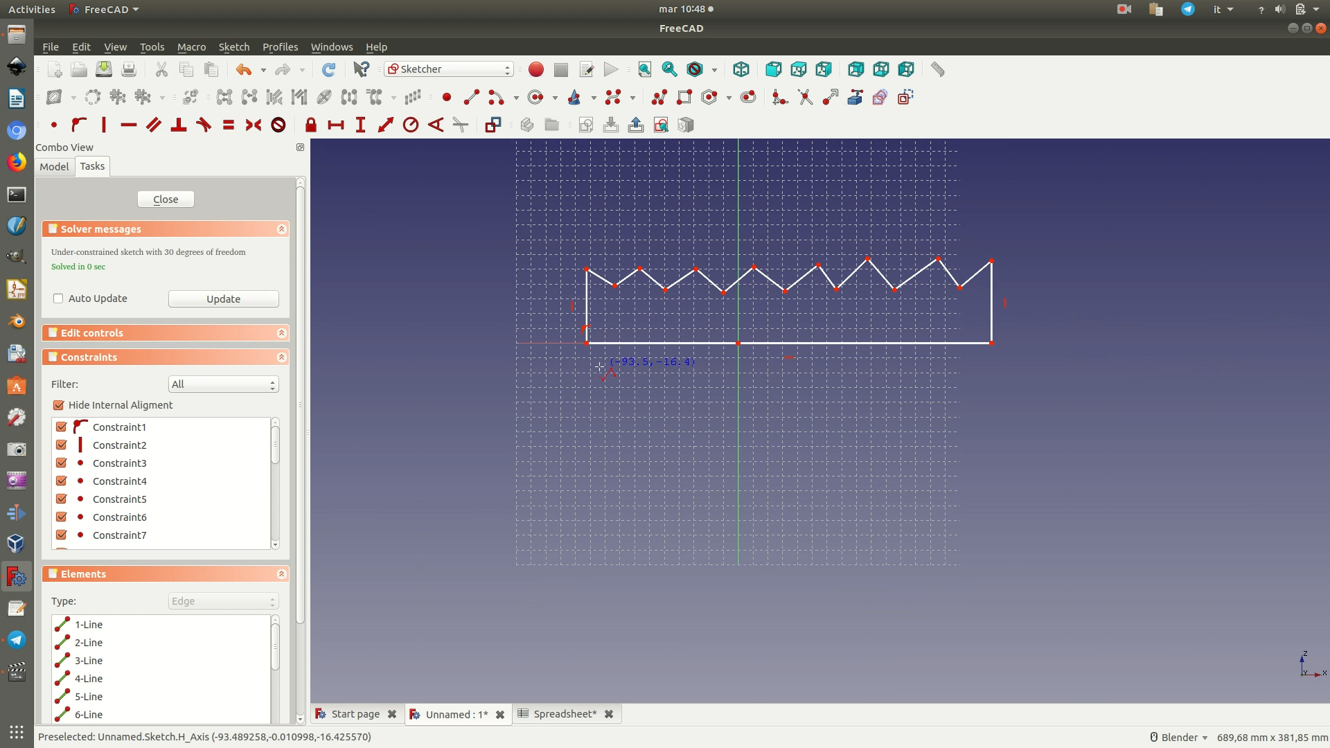
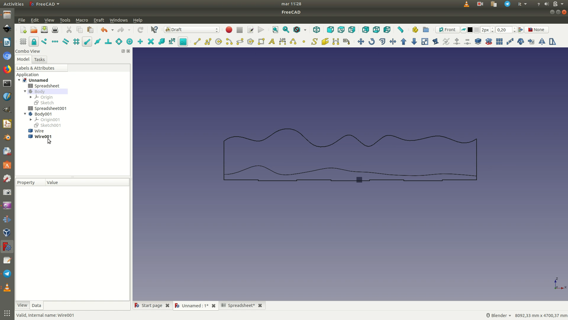
5. Select the Sketcher Workbench. Then, click through the menu Sketch > Sketcher Geometries > Create Polyline. You can now draw a shape similar to that in the image below. The shape should only approximately reflect the structure of your dataset. The number of points on the segments in the top line should be equal to the number of rows in the data, but that's about it: we'll fix everything else further on, from lengths to heights, straightness of lines, distances and the rest. 

Note: to exit the draw mode and finish your shape or lines, you might need to press ESC on your keyboard.

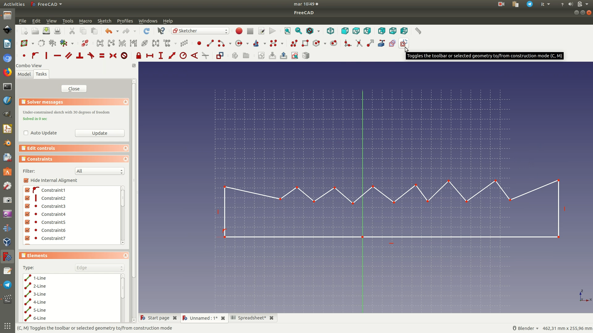
6. The next thing to do is to draw the lines that will serve as guides to position the elements correctly. To do so, you first switch to Construction Mode. Construction Mode allows you to draw lines that are not actually part of the object itself, but that only serve as modeling supports. To switch to Construction Mode, go through the menu Sketch > Sketcher Geometries > Toggle Construction Geometry. 
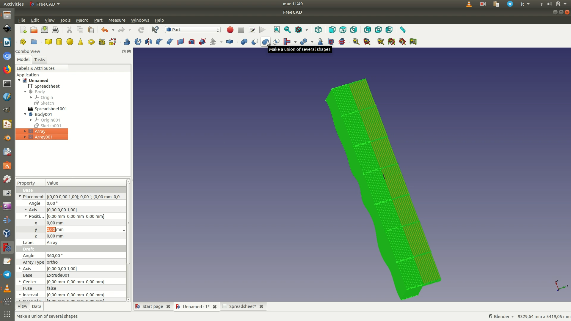
If you have done this correctly, all the lines you now draw will be blue, rather than white. We now draw a grid of lines like in the first image below. 
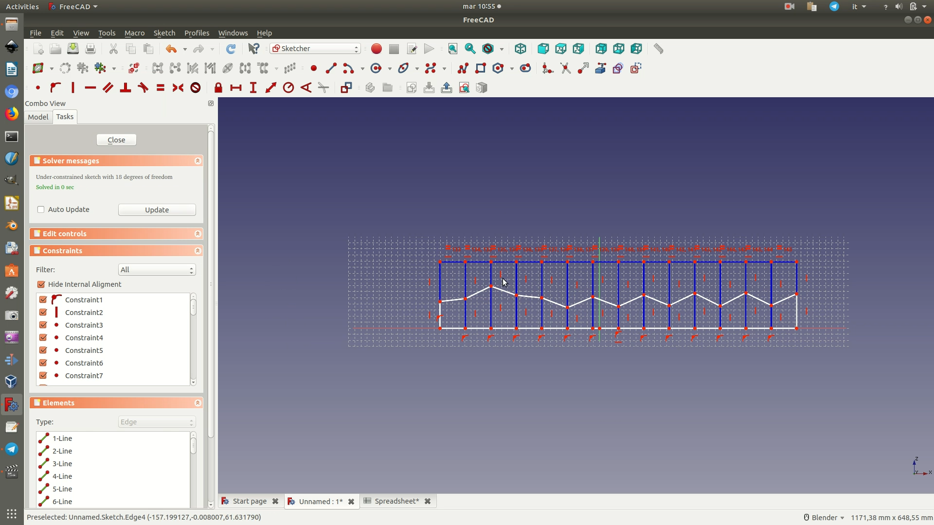
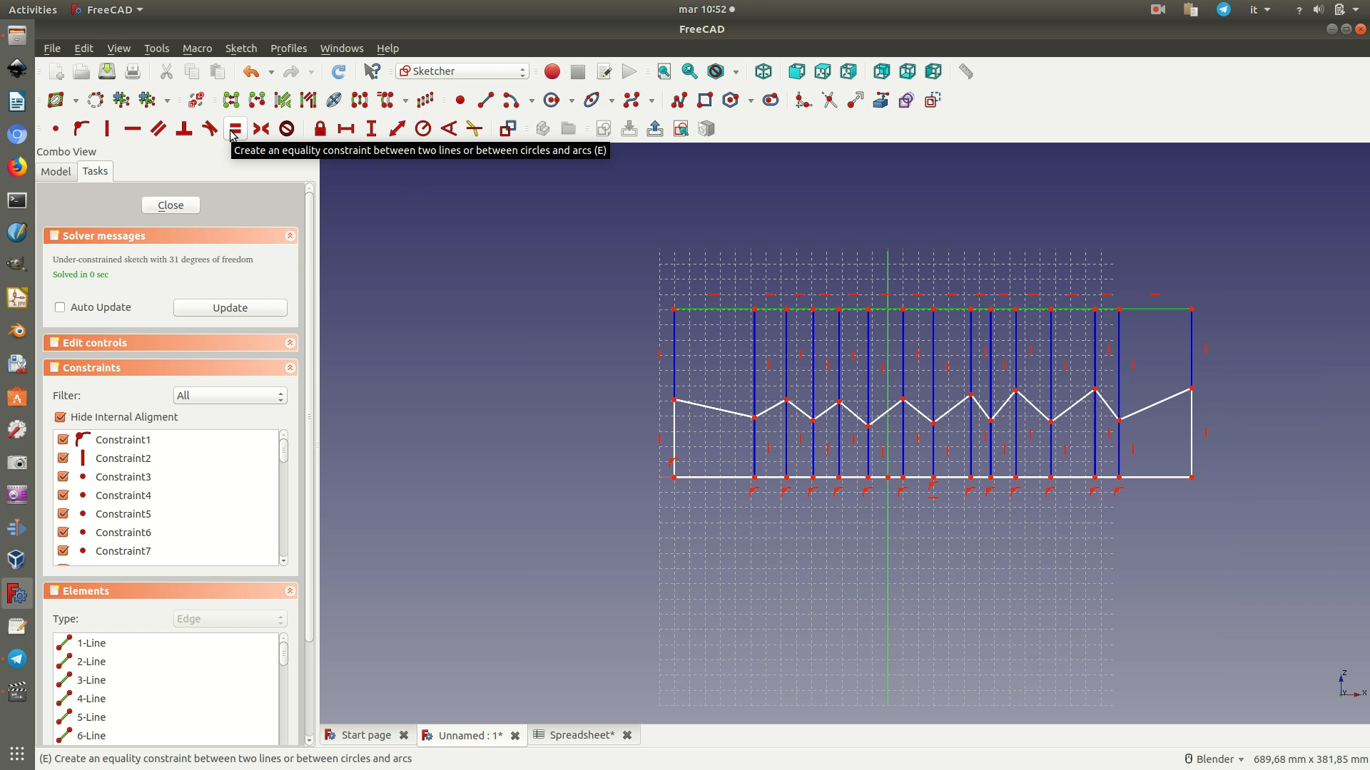
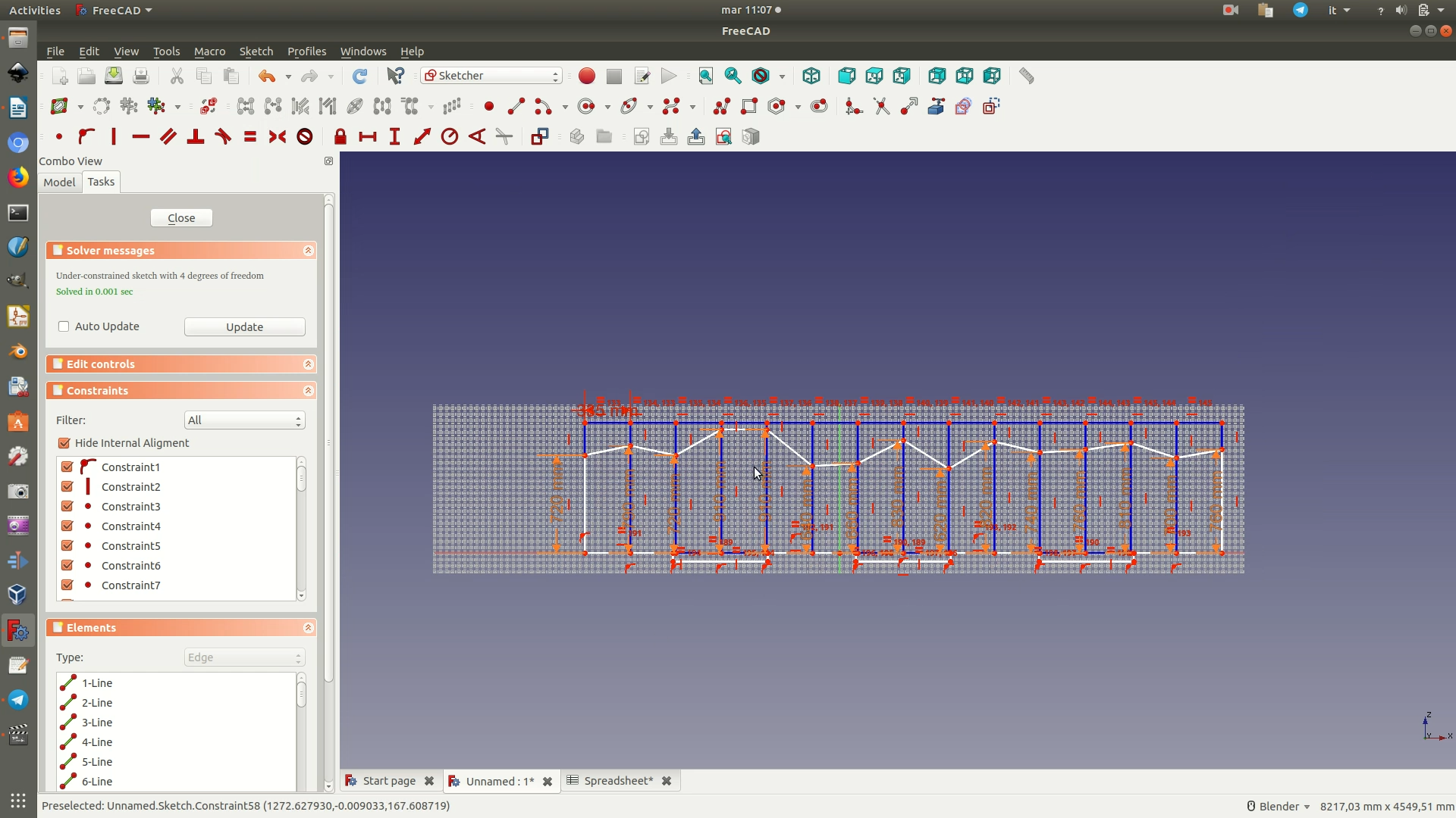
To get there, start by drawing a series of segments running parallel to the base line, each segment starting and ending roughly above the start and end of each segment of the 'line chart'. You can draw such segments by clicking through the menu Sketch > Sketcher Geometries > Create Polyline. You now select all segments by clicking on each of them (selected elements turn green) and then apply the Equality Constraint, so that they are all the same length. The second image below shows you where to find the constraint commands (the Equality Constraint is represented by the red equal sign), otherwise navigate through Sketch > Sketcher constraints > Constrain equal. At this point, you need to draw lines connecting the first point of each of these segments to the first point of each segment of the ‘line chart’. These vertical line are the blue ones you see in the image below. To draw such lines, make sure they start and end on the points of the two segments. You'll know you are in the right start or end spot because the points turn yellow when your cursor is over them. You might also need to zoom in closer to make sure you are connecting them. Just like you had done with the green horizontal lines, you now select all of them and apply a constraint, only this time it is the Vertical Constraint (Sketch > Sketcher constraints > Constrain horizontal ), as you want the line to be a straight line connecting the top segments to the segments in your line chart. To know if the drawing is as it should be, check if all the top horizontal segments have a small red equal sign on the top and a red horizontal bar; and all vertical segments have a small vertical red line at the side, like in the image below. Thanks to this process, all the points in the line chart are at equal distance along the line and you can proceed to bind the data to these points.

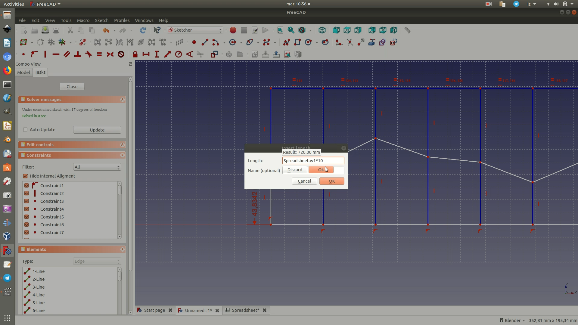
7. You will use a procedure similar to the one of the previous step to make sure that the distance of the points from the base corresponds to the data value they represent. To do this, first of all draw a segment connecting each point of the line chart to the base, through the command: Sketch > Sketcher Geometries > Create Line. You will know the segment is connected to the base if you draw the line until the base segments becomes highlighted in yellow. You then assign to all these vertical lines the Vertical Constraint you used before, as you want the segment to form a straight line connecting the points in the line chart to the base. 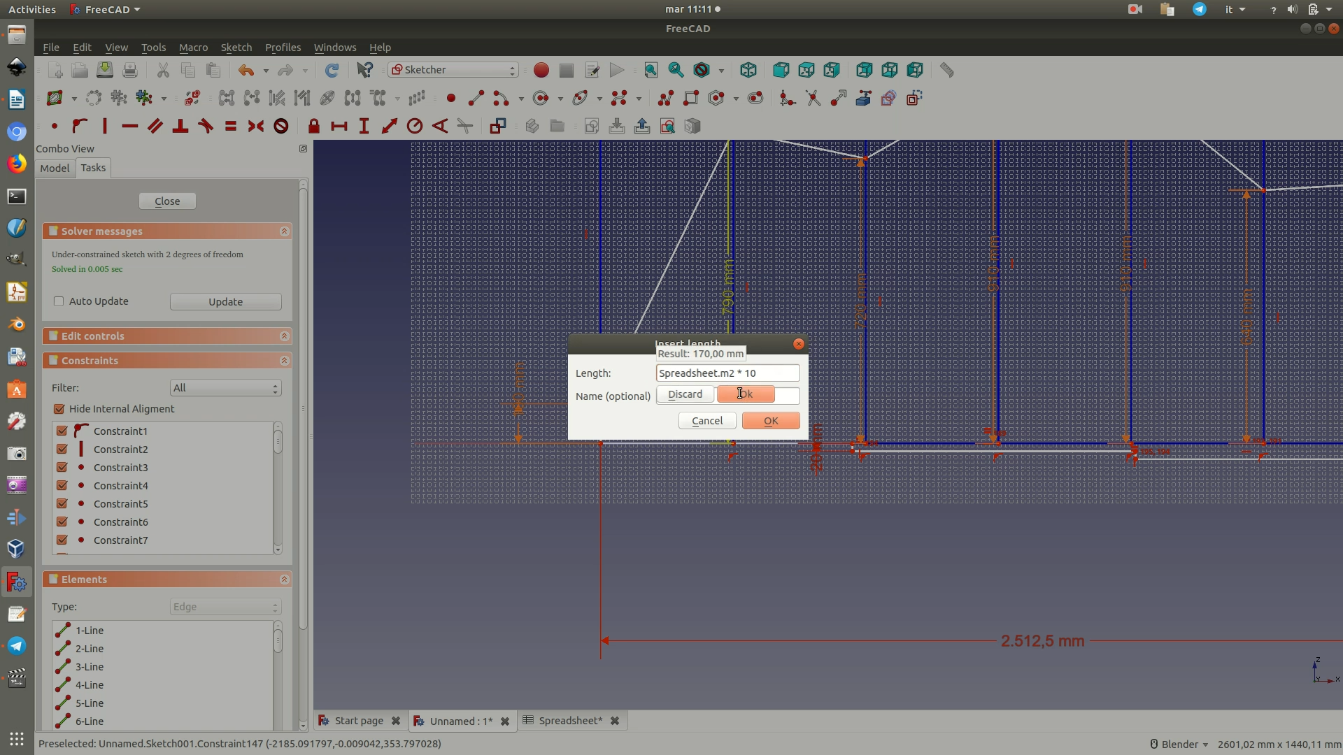Now you assign another constraint to these lines, the Vertical Distance Constraint (Sketch > Sketcher constraints > Constrain vertical distance), as you want these line to be as long as the data value the points represent. You start by selecting the first vertical line on the left and by clicking on the constraint that lets you fix the vertical distance between two points. A pop-up window will now appear asking you the length. Type in the name of the spreadsheet followed by a dot (in this case Spreadsheet.) followed by the alias of the cell that the selected point should stand for (w1 in the image). Note that by default the values in your data are converted to millimeters. If you have very large or small numbers, you might want to scale them by dividing or multiplying all of them by multiples of 10 (or whatever number you wish, as long as all the data points are scaled by the same number). 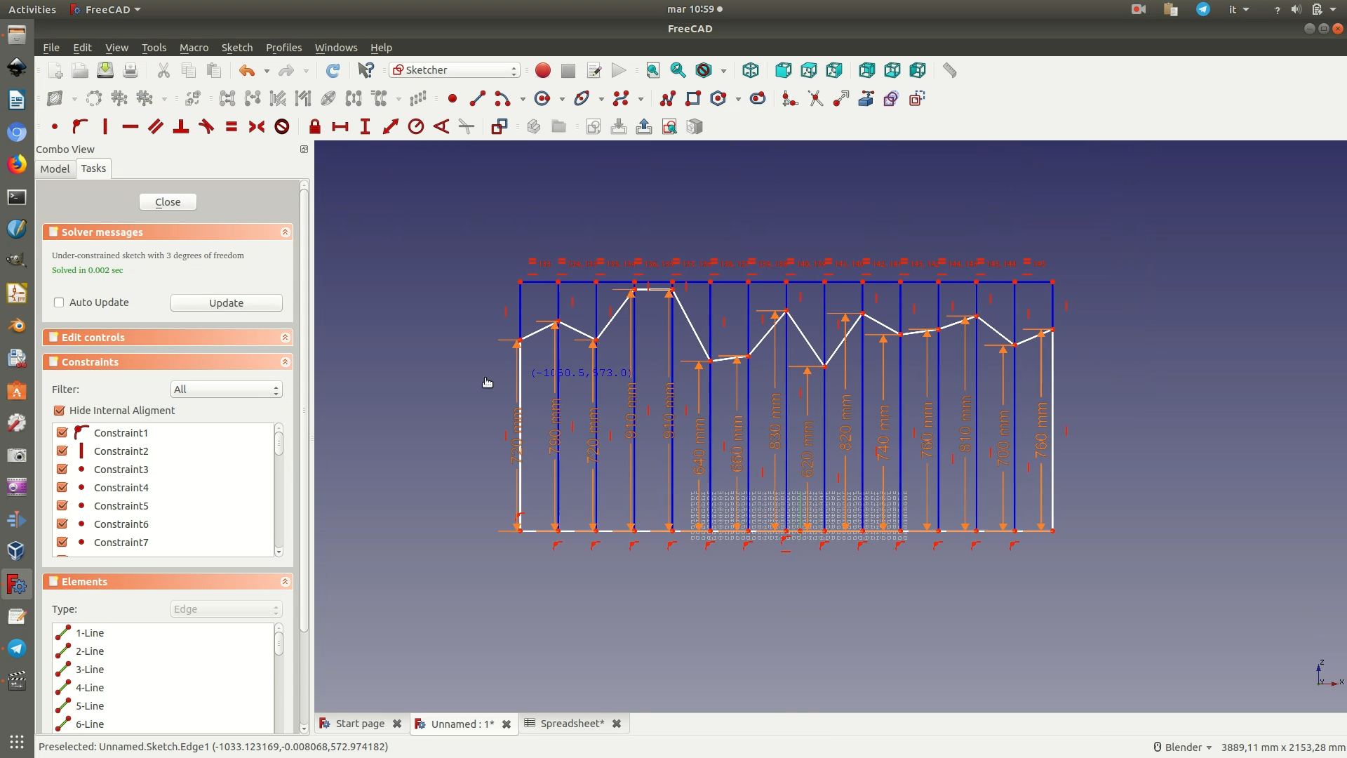You repeat this step for all the row of the dataset/vertical lines of your sketch. The end result will resemble the second of the image below.

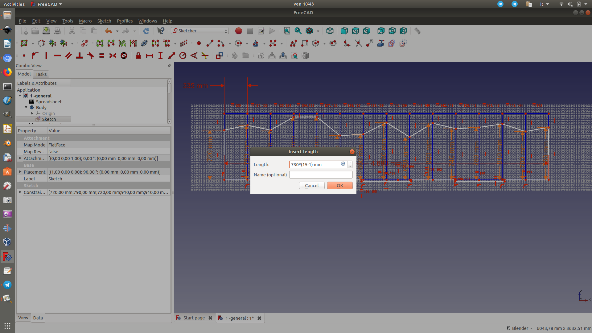
8. Now that you have defined the height of the object, you will define its width. Since this is meant as a walkable object, you want the distance between two points to be roughly the distance of a step (73cm). Of course, this is a rule of the thumb and you will need to come to terms with other constraints, like the amount of space you have available and the number of datapoints in your spreadsheet. For example, if you have few datapoints and want a big object, you will go for a higher number; likewise, if you have many datapoints and need a smaller object, you will go for a smaller number. To set the width, select the base line of the object and click on the Vertical Constraint. In the pop-up that appears, type in 730 * [the_number_of_datapoints - 1].

9. At this point, you will add 3 protruding ridges to the base of your shape. These elements will let you fit the object onto its base, like a puzzle, when you will assemble it. First delete the current base segment. Then, through the menu Sketch > Sketcher Geometries > Create Polyline, draw the shape as shown in the picture, approximately. Thirdly, apply constraints to make the top horizontal lines of the same length (select them and pick Equality Constraint), then the three bottom horizontal lines of the same length (select them and pick Equality Constraint) and finally the vertical lines of the same height (select them and pick Equality Constraint). At this point, you want to make the three ridges of the same height as the depth of the material you are using as a base. In our case, 20mm. To do so, select any one of these short vertical segments, choose the Vertical Distance Constraint and type in a value of 20mm. At this point, you have drawn the basic shape and you can exit the Sketch by clicking through the menu Sketch > Leave Sketch.

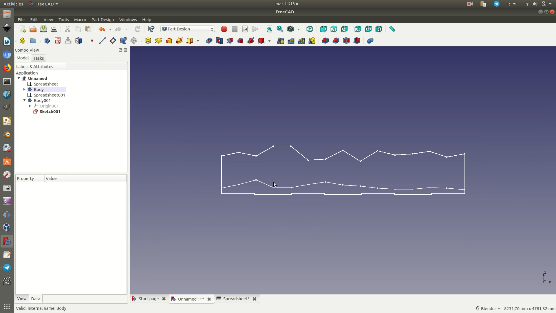
10. Now that you have built the model for representing the first data series, need to create the model for the second data series. Luckily, you don't need to repeat all the steps. Select the Body component from the left sidebar and copy-paste it. Then, right-click on the first Body component from the left sidebar and select Hide Selection. At this point, all you need to do is edit the vertical constraints assigned in point 7 so that they instead match the aliases of the second data series. When you're done, exit the Sketch by clicking through the menu Sketch > Leave Sketch. You can temporarily unhide the first curve again to see the two side-by-side for comparison.

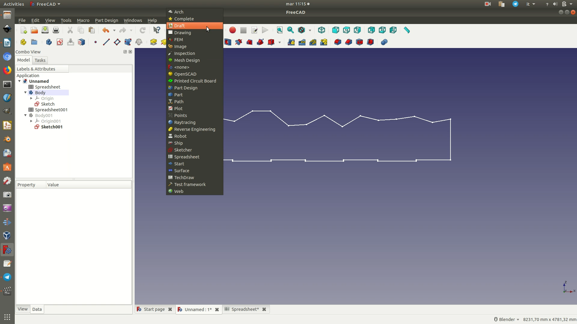
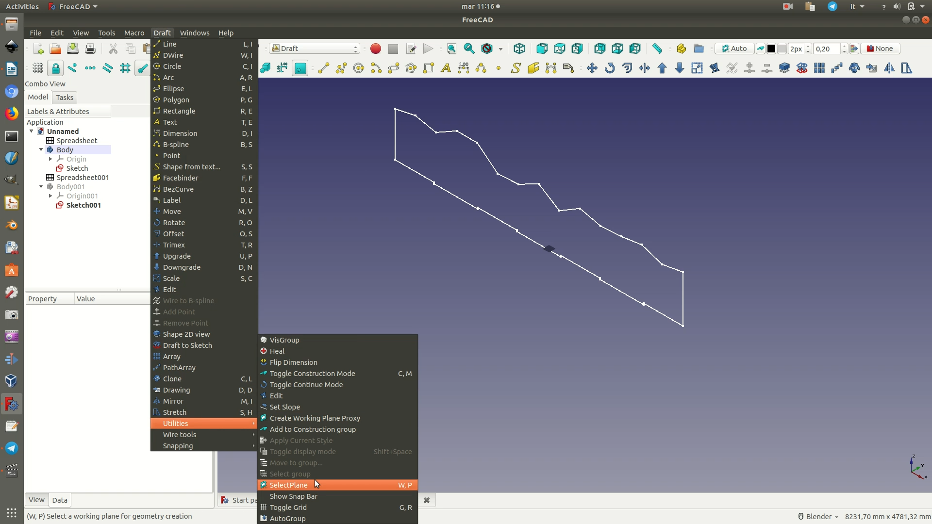
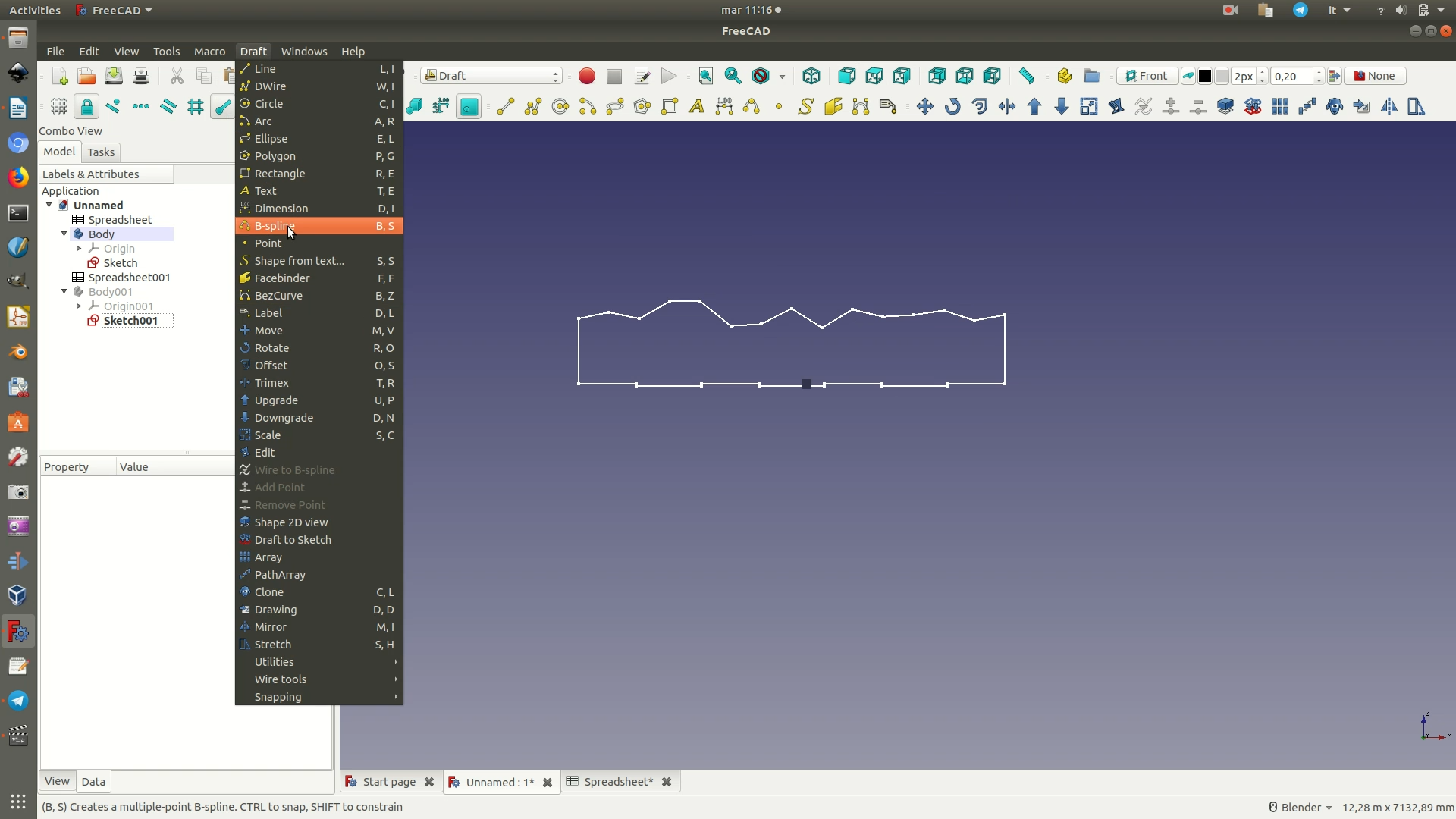
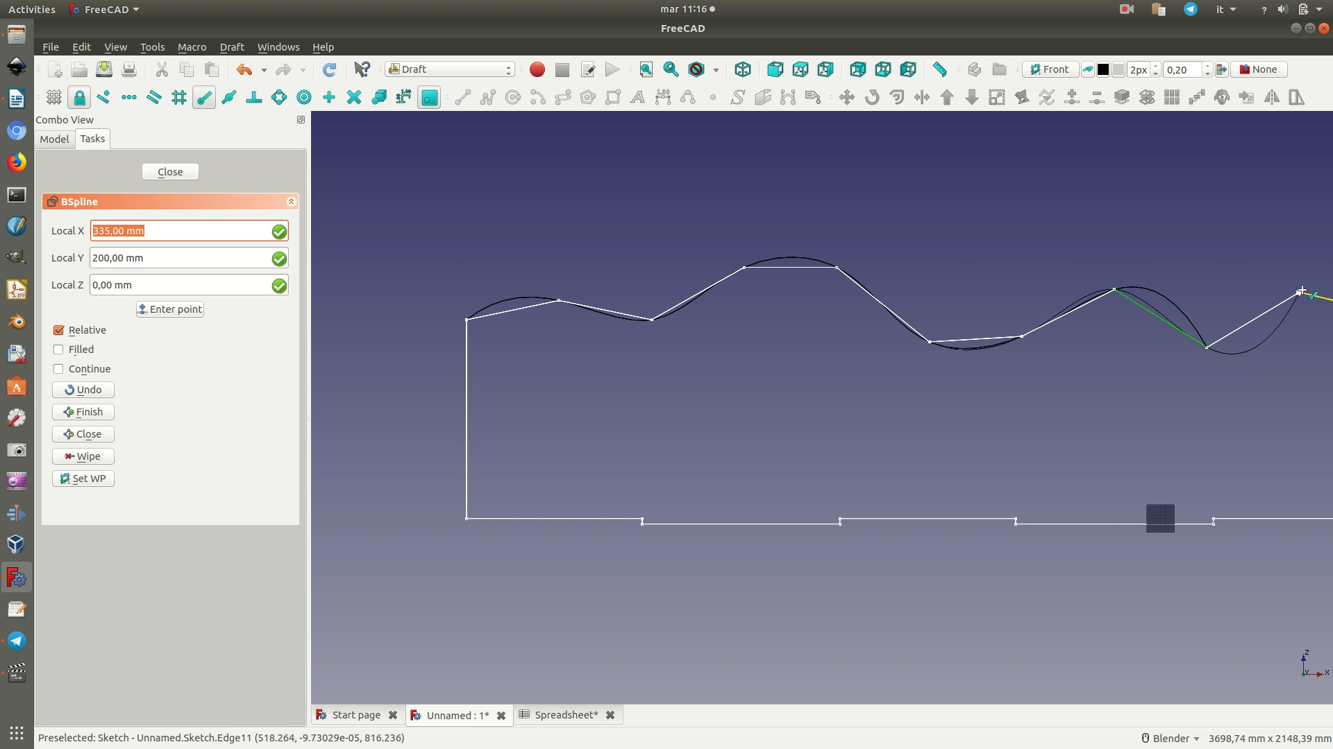
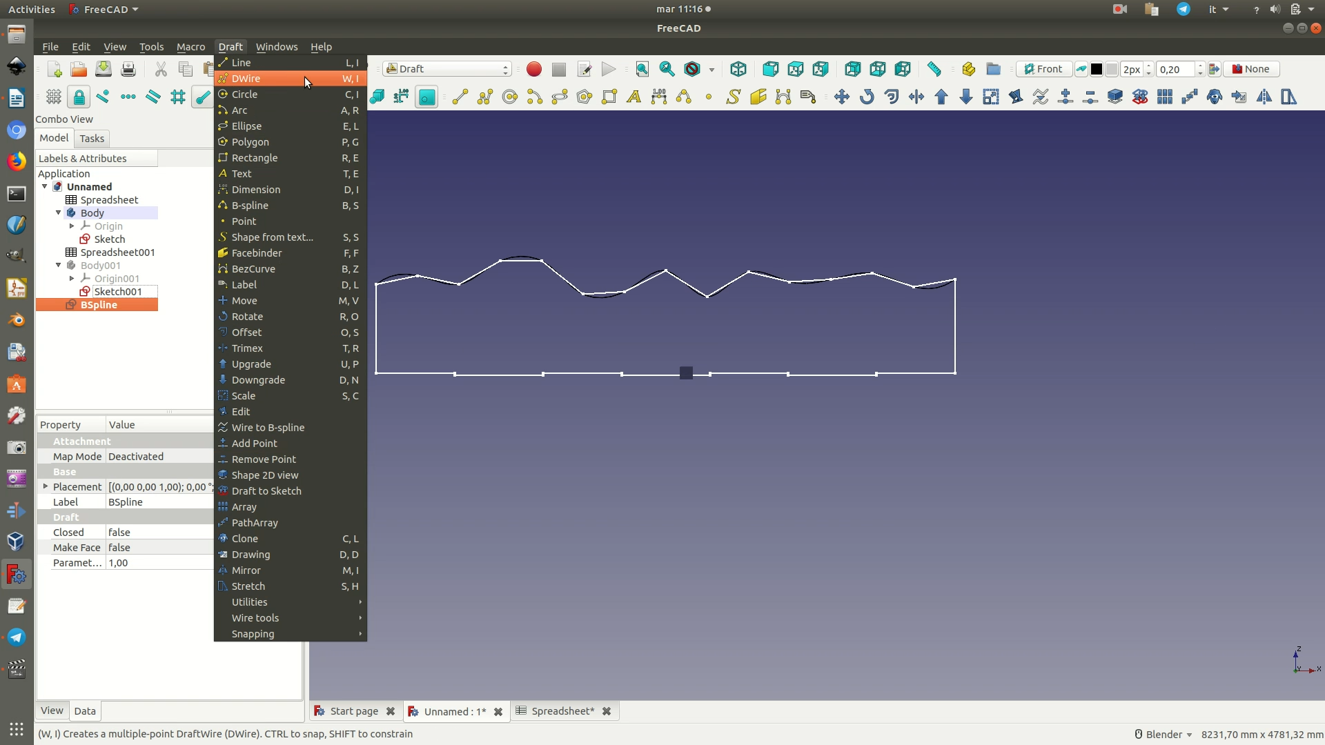
11. Now it is the moment to transform the line charts into a curve - as this will facilitate how people will walk on it. If you prefer to keep the lines straight, you may skip this step. Select the Draft Workbench and then go through the menu Draft > Utilities > Select Plane. This will let you pick which plane to position your bi-dimensional object on. From the panel that appears on the left side, select the XZ plane. To generate the curve, click through Draft > B-spline. At this point, move the cursor so that it is next to the first point of the line chart, that representing the first datapoint, and click. You will know that you are selecting that point because the segment next to it turns orange and small turquoise icon of a point and a line will appear. Move the cursor to the next point and click. Repeat this for all points of the line. Once you are done, hover your mouse over to the left sidebar and click Close from the B-spline panel. Once you’ve drawn this first curve, you need to design the bottom of the object, because the spline you have designed, while it did use the previous lines of the sketch as a guide, is in fact a new object. To complete this spline curve into a polygon, go through the menu and select Draft > DWire. You now move your cursor to complete the shape following the white lines of your sketch, like you did to draw the B-Spline, with the difference that now the lines are straight. 
When you are done, you need to join the two elements (the DWire lines and the B-spline curves) into a single one. To do this, go to the left-hand panel where you see the BSpline element and the DWire elements and select them both (by Shift-click). Then click on the blue arrow icon pointing upwards, or by clicking through the menu Draft > Upgrade. You will know you have achieved this successfully because the left sidebar panel, where before you saw the BSpline element and the DWire elements, now only has a Wire element. Hide this Wire element and the corresponding Sketch element by right-clicking on each and selecting Hide Selection from the menu that appears. Now select the other sketch, the one representing the other data series. It should have been hidden, so right-click on it and select Show Selection from the menu that appears. At this point repeat the drawing of the B-Spline and DWire, and then their Upgrade, like you did for the previous curve.

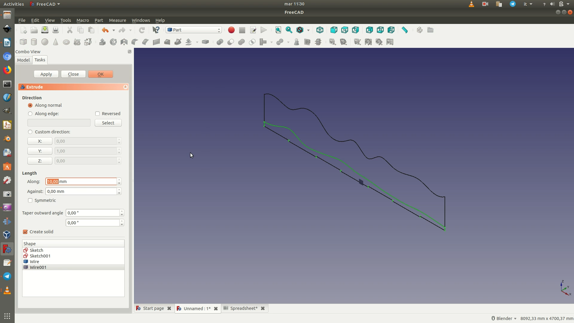
12. In this step, you will transform the curves from bi-dimensional drawings to models of solid shapes. Move to the Part Workbench and then select one of the two Wire objects from the left sidebar. You might want to change the view so that you are able to see the 3rd dimension. To do so, click on through View > Standard Views > Axonometric. Then click through the menu Part > Extrude. On the panel that appears on the left, under Length, type in 20mm and then click OK. This because the curves will be carved out of layers of wood sheets, each being 20mm in thickness. If you are using another material or sheets of another thickness, type in that amount. Repeat this extrusion for the other curve.

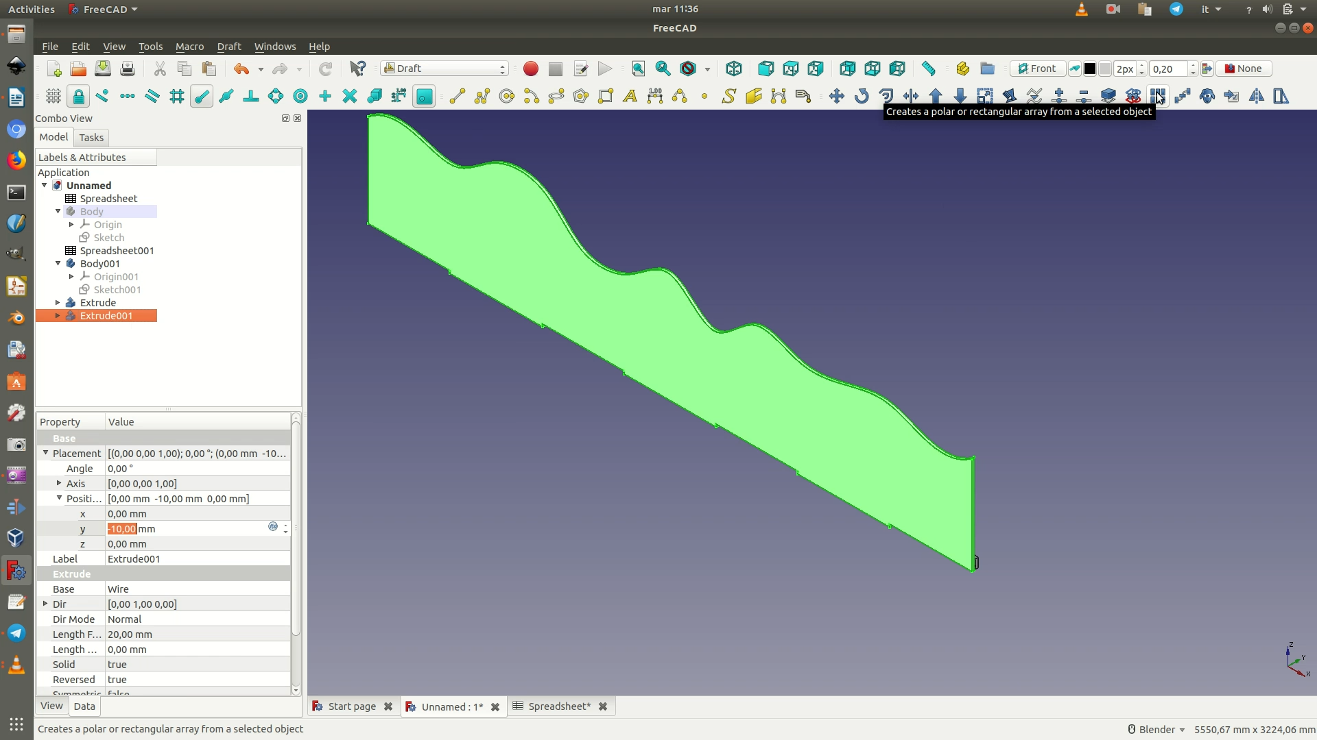
13. In the end, the curve object has to be wide and stable enough so that people can walk on it. To achieve this, the curves will be formed by placing 10 of the 20mm-thick sheets of wood. These sheets will be positioned 10mm apart, so that the object is stable but requires less wood material than a completely full volume. To insert a gap between the curves, switch to the Draft Workbench. On the left sidebar, select the first Extrude element. On the panel below, where you see the buttons View and Data, click on Data. In the grid that appears, open the Placement element and then the Position element nested inside. Once the xyz coordinate values appear (they should all be zero now), type in -10mm for the y.

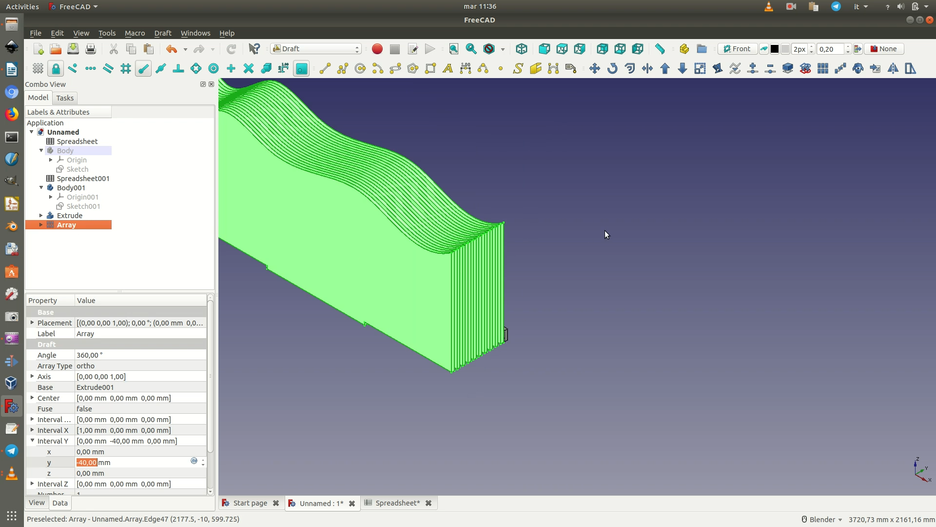
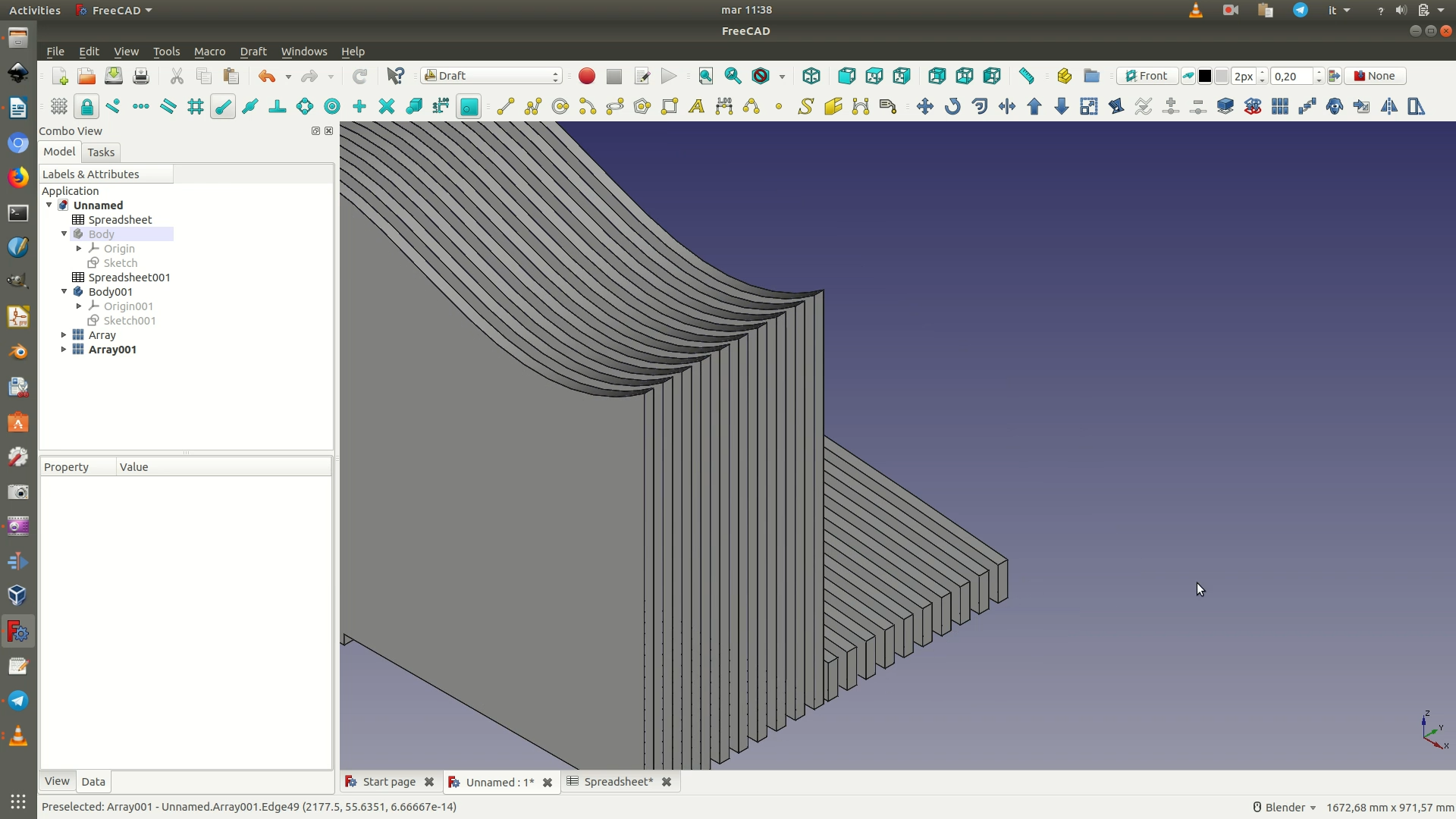
14. On the left sidebar, select again the first Extrude element. Then go through Draft > Array. On the panel below, where you see the buttons View and Data, click on Data, if it’s not already selected. In the grid that appears, change the following variables to match the following values:

• Number X : 1
• Number Y: 10
• Number Z: 1
• Interval Y: -40.00mm¹

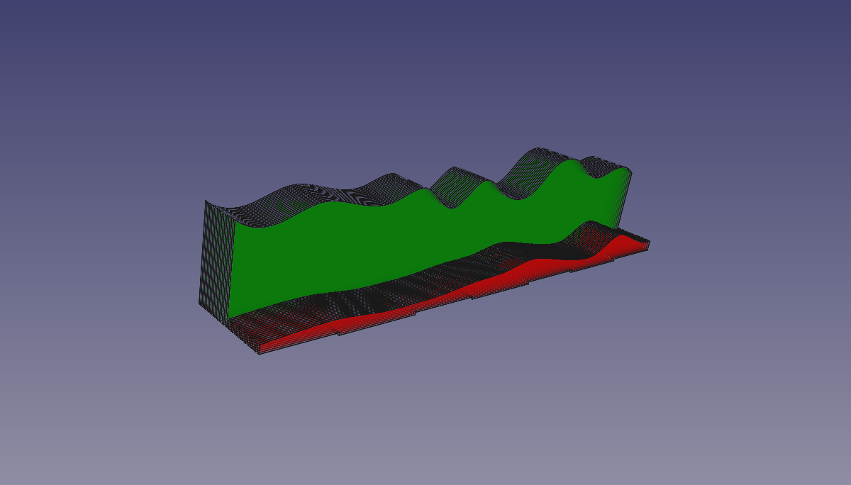
You will now have a series of curve objects like in the picture below. You might want to change the view so that you are able to see the 3rd dimension. To do so, click on through View > Standard Views > Axonometric.
¹assuming you are working with sheets of 20.00mm.

15. Select the second Extrude element and repeat the previous two steps (13 and 14), In step 15, once the xyz coordinate values appear (they should all be zero now), you will need to type 10mm (not -10mm) as the value for the y.
In step 14, when typing in the values for this second Extrude element in the Data panel, change the following variables to match the following values :

• Number X : 1
• Number Y: 10
• Number Z: 1
• Interval Y: 40.00mm¹ (not -40.00mm)

You will now have a series of two curve objects like in the picture below. You might want to change the view so that you are able to see the 3rd dimension. To do so, click on through View > Standard Views > Axonometric.
¹assuming you are working with sheets of 20.00mm.

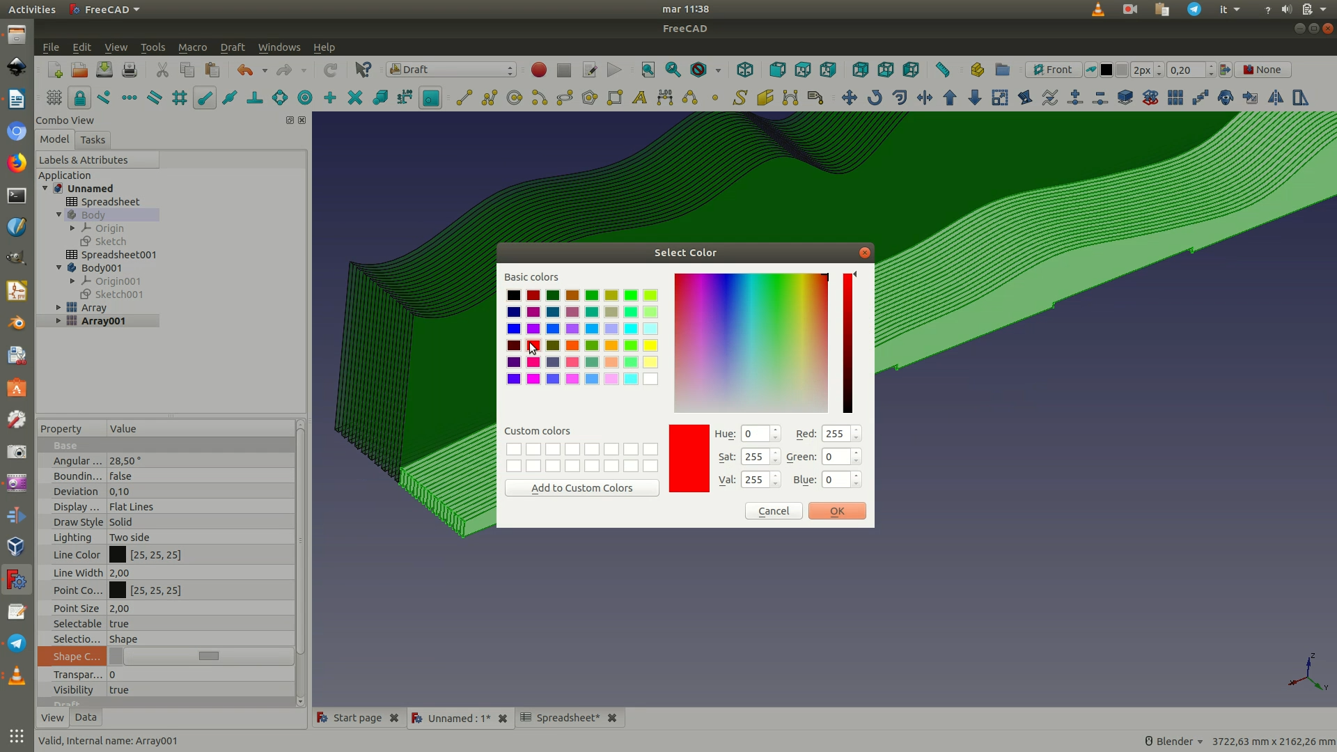
16. To make it easier to work on the two curves without confusion, and to get a clearer image of the possible final effect, you can color the two curves with distinct colors. This step does not have any implication on the design, it is just a visual effect that is useful during the 3D modeling session. On the left sidebar, click on the first Array element. On the panel below, where you see the buttons View and Data at the bottom, click on View. In the grid that appears, you will see a variable called Shape Color. Edit it by selecting a color to your liking. Below Shape Color, there is the variable Transparency. Type in a value lower than 100 (for example 50), so that you will be able to see both curves even when one is in front of the other. Do the same for the second Array element.

17. Switch back to the Part Workbench. Select both Array elements from the left panel and join them into a single object by going through the menu Part > Boolean > Union. You will see that this has been carried out correctly because you now have a single Fusion element in place of the two different Array elements. When selecting the Fusion element from the left sidebar, you will also notice that the whole object, with both curves, gets selected.